How to order stuff

Vanilla NNs with fully connected layers work by each neuron receiving all the outputs of the previous layer (or the inputs in the case of input layers) and then doing calculations over them and the weights and biases of the given neuron. This works well in general, but is especially good when each input value has a specific meaning, e.g. [<number of cats>, <number of dogs>, <number of mice>, ...].

In the case of images, translating the pixels slightly left won’t change the overall picture, but it means that you can’t assume that pixel (123, 433) is always part of an eye. That is to say, for images, it’s more important to focus on the position of inputs relative to other inputs, rather than the absolute position in the input vector.

This is the main innovation introduced by convolution networks. They work on chunks of (usually) pictures, looking for interesting stuff in a small subsection of the whole image. Then the next layer also looks over small subsets. And so on, each time lowering the dimensionality of the previous layer, until it gets to the final fully connected layer(s).

Chunking pics (local receptive fields)

The input image gets split into a load of small (e.g. 5x5 pixel) chunks. These then get fed into a kernel or filter, which is nothing more than a known similar sized matrix. The result of feeding the chunk into the filter is a single number, which is the output of that chunk/filter operation. The magic trick here is that the same filter is used for every single chunk, resulting in an output matrix for that filter. Then the same thing happens for the next filter. And the next. This process results in a set of output matrixes, one for each filter.

The image chunking algorithm is pretty much for each pixel, take a square of the surrounding pixels, as seen below:

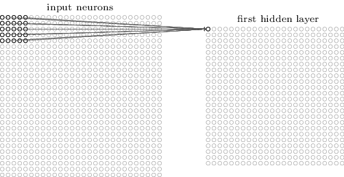
Of course that will only work if there are pixels to each side of the current pixels, so you either start away from the edge, or pad the image with extra (0) pixels for it to have something to work with.

These chunks are called local receptive fields.

Another thing worth mentioning is that these chunks are overlapping (unless the step is larger than the chunk size). This is because the surroundings of each pixel get processed, as opposed to just segmenting the image into disjoint areas and processing each area. Because the chunks are overlapping, the resulting matrix of filtered values is the same size as the input image (assuming a step of 1 and zero-padding on the margins). Larger step sizes, or no padding will of course result in smaller output matrixes.

Output volume size

The size of the output volume can be calculated with: $$\frac {(W - F + 2P)}S + 1$$ where $W$ is the size of the input volume, $F$ the size of the filter, $S$ the step, and $P$ the amount of zero padding on the margins.

Convolutions

This is where the convolutions name comes from. The operation here is to transform the image by convolving it with a filter, just like if it was doing a basic blur operation or something.

One thing that caught me was that in all the tutorials the convolution is presented by $\text{chunk } \cdot \text{ filter}$, but the actual convolution equation is $\text{chunk } \cdot \text{ filter}^T$. It all works out in the end, but simply thing of the filter going into the convolution as $\text{ filter}^T$, which gives $\text{chunk } \cdot \text{ filter} = \text{chunk } * \text{ filter}^T $

Filters

Seeing as the filters are applied to every chunk, to get a set of transformed images, all that is needed to represent each filter is an n-by-n matrix of weights + a bias. That is, each filter can be represented by the following (with a couple of index adjustments, etc.): $$a_{j,k} = \sigma \begin{pmatrix} b + \sum_{l=0}^n \sum_{m=0}^n w_{l,m}a_{j+l,k+m} \end{pmatrix}$$ This is nice, as it drastically lowers the number of weights, seeing as each layer will have $\text{number of filters} \cdot (n^2 + 1)$ weights, as opposed to the <number of inputs> * <neurons in layer> of a fully connected layer. To use another image from Neural Networks and Deep Learning, the following is a diagram of what a layer with 3 filters would result in:

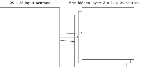
In this case the input image wasn’t zero-padded, so the convolutions shrink the image by their margins.

Filters can be viewed as detecting various features in the input image, e.g. edges, corners, gradients, etc.

Pooling layers

After filtering, the next step is to downscale the filter results, in order to work on fewer dimensions. This is pretty much the same as in the previous layers, but instead of overlapping chunks, it splits the output into areas e.g. 2x2 and runs another filter over them, as shown below:

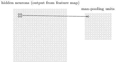
These areas are disjoint, and will downsize the inputs by the size of each area, e.g. pooling with regions of 2x2 will result in an output with an area 4 times smaller than the inputs area. This can be viewed as saying whether the given feature was found in that area - in most cases it’s a lot more important to know whether it was there than its precise position.

Pooling function

Different functions can be used for pooling. The most common seems to be a simple $max()$ over the values of the chunk, but other candidates are simple averages or L2. $max()$ seems to work the best for now.

Normalization layer

Many types of normalization layers have been proposed for use in ConvNet architectures, sometimes with the intentions of implementing inhibition schemes observed in the biological brain. However, these layers have since fallen out of favor because in practice their contribution has been shown to be minimal, if any.

Fully connected layers

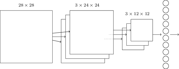
The general architecture of a convolution network is INPUT -> [[CONV -> RELU]*N -> POOL?]*M -> [FC -> RELU]*K -> FC, where FC is a fully connected layer at the end, which works on the most important features found in the previous steps:

Backpropagation

Fully connected layers

Same as for vanilla NNs

Pooling layer

In the case of max pooling, the only one that contributed anything is the selected value, giving that value. This means that $$\frac {\partial C}{\partial z} = \begin{cases} \text{1 if z selected} \ \text{0 if z not selected} \end{cases}$$

ReLu layer

Seeing as this is the same as max pooling, but with only 2 items, the gradient is $1$ if the input was positive, otherwise it’s $0$

Convolutional layer

This one is more fun. The gradient is also a convolution: $$\frac {\partial C}{\partial a_i}= F^T*\delta_{i+1}$$ where $F$ is the filter used, and $\delta_{i+1}$ is the gradient from the next layer.